Access via: SPRING Calculation Model calibration (gradient method)…

Once a groundwater model has been created, i.e. all known or estimated parameters and boundary conditions have been entered, a model calculation usually brings together all the individually determined data for the first time. As many influencing variables are only estimated, there are usually deviations from a measured groundwater condition. Once all conspicuous incompatibilities (incorrect extraction, boundary conditions, etc.) have been eliminated, the K value is normally the most uncertain variable.

When calibrating with the gradient method, the hydraulic conductivity values of the elements - starting from an initial value - can be changed iteratively so that a measured groundwater surface is recalculated as accurately as possible. The following model types can be processed:

• 2D horizontal models

• 2D/3D models

• 3D models

As the calibration is carried out using steady state calculations, it is crucial to use a target state that is as steady state as possible! The target state created must be free of contradictions, i.e. the gradients determined must always correspond to the general flow direction. Otherwise, nonsensical hydraulic conductivity values may result. Particular caution is required in the case of springs and valleys as well as watersheds.

The target state is defined by the calibration potential heads (attribute EICH). The EICH attribute must be defined for each node. To consider all groundwater-influencing data, please refer to the "Interpolation of groundwater contour maps".

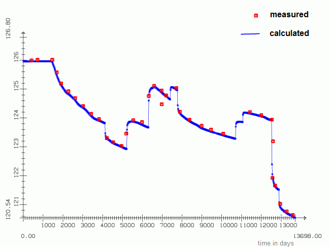
Example of a transiently calibrated hydrograph

Calibration using inverse modelling is described in a later chapter.

Iterative calibration of the horizontal K-values